Multiple Importance Sampling

Next Event Estimation (NEE) struggles with scenes that have huge light sources. Most of the light samples end up insignificant, and the result is a lot of noise. In this post I look into combining NEE with BSDF-based sampling to get the best of both worlds.

Why NEE fails

Sampling the light sources is done with a uniform distribution, meaning that every small patch of the light source has the same chance of being selected. This makes sense, we have no prior knowledge about which part of the light contributes most. Currently I only support diffuse emission and one material per object, so this uniform strategy is proportional to the emission distribution of the light source.

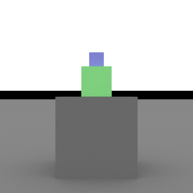
The issue is when a light source is very large, most of its surface does not contribute much to the resulting image:

NEE fails in this case

Here NEE has a large chance of selecting a sample like $S_1$, which is far from the object, instead of one like $S_2$ that is close. Not only is the average distance large, but the viewing angle tends to be glancing too, meaning the geometric factor is tiny, resulting in amplified noise. Samples are effectively wasted on unimportant parts of the scene.

In this case however, the BRDF-based backwards tracing I used earlier would shine, since it naturally samples directions that are more visible from the surface.

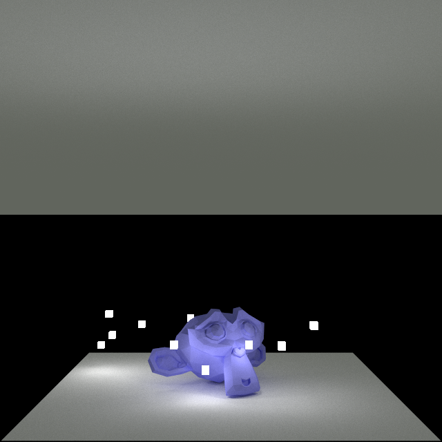
Rendering a scene with an enormous overhead light shows this well:

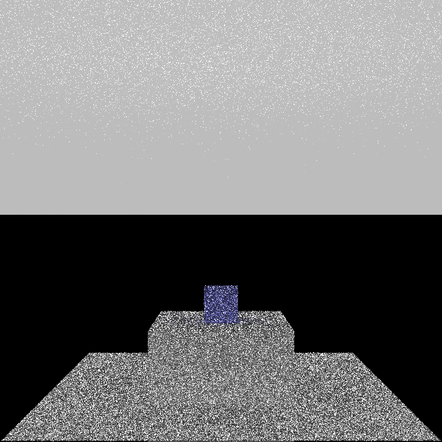
Both images were made with the same number of ray casts.

Multiple Importance Sampling (MIS)

To combine the two techniques, I could just average the two results. This, however, would increase variance in many cases. To properly combine sampling strategies, I need a method called Multiple Importance Sampling. I am largely implementing this based on the Stanford Computer Graphics notes Chapter 9.

The core idea is to weight each technique’s contribution based on how confident it is about that particular sample. In the paper the general form of a multi-sample estimator $F$ is given:

$ \begin{aligned} F = \sum_{i=1}^{n}\frac{1}{n_i}\sum_{j=1}^{n_i}w_i(X_{i,j})\frac{f(X_{i,j})}{p_i(X_{i,j})} \end{aligned} $

In my case I have two estimators ($n=2$) and I distribute the samples evenly ($n_1 = n_2$). Denoting the number of samples as $N$ I have:

$ \begin{aligned} F = \frac{1}{2N}\sum_{j=1}^{N}\left(w_1(X_{1,j})\frac{f(X_{1,j})}{p_1(X_{1,j})}+w_2(X_{2,j})\frac{f(X_{2,j})}{p_2(X_{2,j})}\right) \end{aligned} $

Where the 1-indexed terms ($p_1$, $w_1$) belong to NEE sampling and the 2-indexed terms ($p_2$, $w_2$) belong to the BSDF technique.

The central question of Multiple Importance Sampling is choosing the right weighting functions $w_i$ such that the resulting variance is minimized in the estimator, i.e. there is less noise in the rendered image.

A key detail here is that the weighting functions depend on the sample itself, specifically, they can use the PDFs of both techniques evaluated at that sample. This lets the combination give higher weight to the technique that is more “confident” about a given sample. There are many valid choices for $w_i$. I use the Power heuristic because it is simple and near-optimal in practice. Given that I use the same number of samples per technique, it is defined by:

$ \begin{aligned} w_i = \frac{p_i^\beta}{\sum_k{p_k^\beta}} \end{aligned} $

I use $\beta=2$ in the renders in this article.

Code changes

There’s a lot going on in the sampling and combination code, so let’s walk through it piece by piece:

if (const auto *diffuse_material = std::get_if<DiffuseMaterial>(&material)) {
    color = color + misWeightedEmission(
        diffuse_material->emission, vertex->total_throughput,
        prev_bounce_specular, path_pdfs
    );

    path_pdfs = MisPdfs{
        .bsdf_pdf = 0,
        .nee_pdf = 0,
    };

    if (next_vertex != path_end) {
        path_pdfs = computeNextBounceMisPdfs(*vertex, *next_vertex, materials, info);
    }

    LightSample light_sample = samplePointOnLights(objects, light_table, rng);
    const auto *light_material = std::get_if<DiffuseMaterial>(&materials[light_sample.mat]);

    const auto nee_pdf_bsdf = cosineWeightedHemispherePdf(vertex->p, light_sample.p, vertex->n);
    const auto nee_pdf_nee = light_sample.pdf * areaToSolidAngle(vertex->p, light_sample.p, light_sample.n);

    const auto Ld_nee = evaluateDirectLighting(
        vertex->p, vertex->n, diffuse_material->diffuse_reflectance,
        light_sample, light_material->emission, objects, info);

    if (nee_pdf_nee + nee_pdf_bsdf > 0)
        color = color + Ld_nee * vertex->total_throughput * powerHeuristic(nee_pdf_nee, nee_pdf_bsdf);

    prev_bounce_specular = false;
}

Breaking it down:

misWeightedEmission: Handles the BSDF sampling part, it calculates the weighted contribution of that technique.
computeNextBounceMisPdfs: Calculates the PDFs of both techniques for the next vertex on the path
samplePointOnLights: Draws a sample point on a light source, with a PDF proportional to the radiant emittance of the light sources. It also calculates the PDF of choosing that point.
evaluateDirectLighting: Calculates the NEE contribution.

These functions can be implemented following the formulas in the paper, so I will not share the code in detail. It can be found in the GitHub repo.

One interesting detail I do want to look into is samplePointOnLights. This function needs to first choose a light source, then a triangle from that object and then generate a random sample on the triangle:

#pragma nv_exec_check_disable
LightSample samplePointOnLights(
    std::span<const TriangleMesh> objects,
    std::span<const AliasEntry> light_table,
    Rng &rng)
{
    const auto [object, object_pdf] = sample(light_table, rng);

    const auto tris_table = std::span{object.tris_sampler, object.tris_count};
    const auto [triangle, triangle_pdf] = sample(tris_table, rng);

    const auto p = uniformTriangleSample(triangle, rng);

    return LightSample{
        .p = p * object.s + object.p,
        .pdf = object_pdf * triangle_pdf / world_triangle_area,
        // ...
    };
}

I am using the Alias Method for drawing custom weighted samples in constant time for both the emissive objects and the triangles. Each object has its own sampling table. The weights are proportional to the total irradiance of the objects/triangles, this way the samples are distributed in proportion to the emitted light and sample the source efficiently.

The specular bounce is still handled the same way as before, prev_bounce_specular stores whether the last bounce was specular, meaning the NEE sample would be meaningless.

Results

Combining the two methods yields pretty good results in both cases where one was failing. The scene with the large overhead light that is noisy with NEE now looks as good as before:

Meanwhile using several small cube lights in the Cornell box also look good:

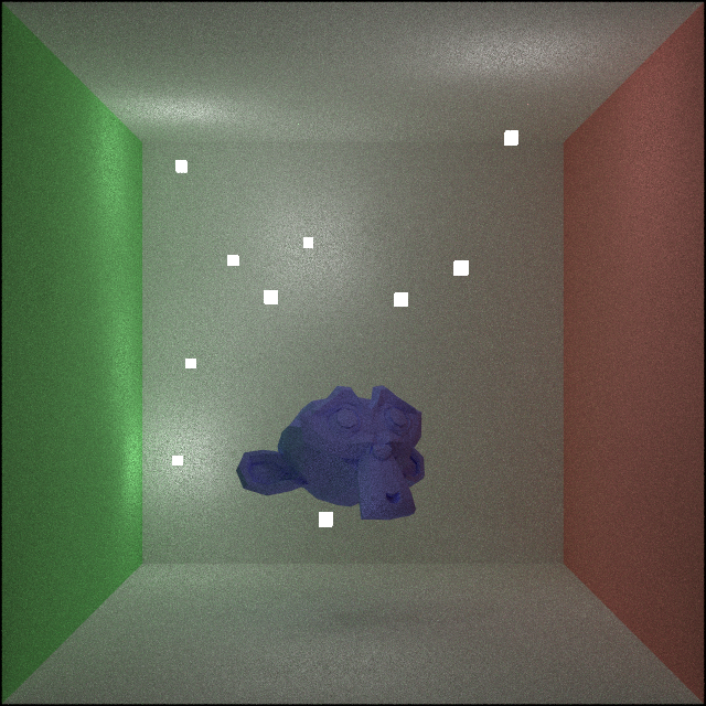
In both cases the same amount of rays were cast for equal comparison.

Conclusion

Combining the two techniques was surprisingly hard, a lot of small details could and did go wrong and debugging a noisy or simply too dark image is never trivial. But the payoff is real: the renderer now handles both large area lights and small point-like sources gracefully, without having to choose a strategy per scene.

I want to speed up these renders, so next I will look into using bounding volumes to cut intersection tests short.

Why NEE fails#

Multiple Importance Sampling (MIS)#

Code changes#

Results#

Conclusion#

Why NEE fails

Multiple Importance Sampling (MIS)

Code changes

Results

Conclusion