Increasing the maximum path length results in more and more sparkles showing up on my renders. Today I explore why that is and how to fix it.
Sampling Distribution
During path tracing the light ray’s path is incrementally built by randomly choosing a new direction and shooting a ray from the last vertex of the path. Wherever that ray intersects the scene geometry is where the next vertex will be.
The key word here is randomly. Recall that the Monte Carlo integration used here can be understood as a simple weighted average of samples:
$ \begin{aligned} I = \sum_i{\frac{g(x_i)}{p(x_i)}} \end{aligned} $
Where $g$ is describes how much light is transmitted in the chosen direction and $p$ is the probabilty density function of the sampling function. The choice of $p$ greatly influences the quality of the estimation.
Looking at a single sample:
$ \begin{aligned} I(\omega_i) = \frac{f(x,\omega_o,\omega_i)L_i(x,\omega_i)cos(\theta_i)}{p(\omega_i)} \end{aligned} $
This equation describes the amount of light forwarded towards $\omega_o$ at $x$ from direction $\omega_i$. Since I am working with diffuse materials only for now $f(x,\omega_o,\omega_i) = \frac{\rho}{\pi}$ where $\rho$ is the albedo of the material. Thus:
$ \begin{aligned} I(\omega_i) = \rho L_i(x,\omega_i)\frac{cos(\theta_i)}{\pi p(\omega_i)} \end{aligned} $
Uniform Random Hemisphere Sampling
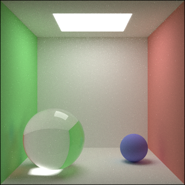
As an easy first approach I used uniform hemisphere sampling for $p$. However, when I let the number of vertices go up to, say, 100, I noticed sprakling noise showing up on my renders.
I figured printing the path vertifces might help.
Extreme limunance path:
    Vertex 1: 0.385328,-0.500000,1.541842, transmission_luminance: 1.000000
    Vertex 2: 0.500000,-0.344371,1.559557, transmission_luminance: 1.443030
    Vertex 3: -0.038083,0.455076,2.500000, transmission_luminance: 0.493101
    Vertex 4: -0.080915,0.500000,2.245682, transmission_luminance: 0.862270
    Vertex 5: -0.081183,0.499000,2.245070, transmission_luminance: 1.286353
    Vertex 6: -0.081017,0.500000,2.245138, transmission_luminance: 2.531174
    Vertex 7: -0.080851,0.499000,2.246114, transmission_luminance: 3.220562
    Vertex 8: -0.079753,0.500000,2.244053, transmission_luminance: 2.513673
    Vertex 9: -0.079602,0.499000,2.243173, transmission_luminance: 3.360210
    Vertex 10: -0.079154,0.500000,2.241265, transmission_luminance: 3.029609
    Vertex 11: -0.080174,0.499000,2.240675, transmission_luminance: 3.507682
    Vertex 12: -0.078747,0.500000,2.239985, transmission_luminance: 3.716078
    Vertex 13: -0.079005,0.499000,2.239519, transmission_luminance: 5.888573
    Vertex 14: -0.080349,0.500000,2.239135, transmission_luminance: 6.807854
    Vertex 15: -0.079568,0.499000,2.238842, transmission_luminance: 9.369415
    Vertex 16: -0.079457,0.500000,2.238765, transmission_luminance: 18.565853
    Vertex 17: -0.079790,0.499000,2.238041, transmission_luminance: 26.037645
    Vertex 18: -0.081577,0.500000,2.237849, transmission_luminance: 25.126522
    Vertex 19: -0.080918,0.499000,2.235405, transmission_luminance: 16.476456
    Vertex 20: -0.081494,0.500000,2.236084, transmission_luminance: 24.503897
    Vertex 21: -0.081538,0.499000,2.237195, transmission_luminance: 29.325005
    Vertex 22: -0.082457,0.500000,2.237414, transmission_luminance: 42.426514
    Vertex 23: -0.083173,0.499000,2.237584, transmission_luminance: 61.283707
    Vertex 24: -0.082742,0.500000,2.237409, transmission_luminance: 110.944992
    Vertex 25: -0.079831,0.499000,2.236013, transmission_luminance: 58.542580
    Vertex 26: -0.080743,0.500000,2.236105, transmission_luminance: 85.939781
    Vertex 27: -0.079277,0.499000,2.236310, transmission_luminance: 85.985481
    Vertex 28: -0.078363,0.500000,2.235018, transmission_luminance: 91.193588
    Vertex 29: -0.078848,0.499000,2.235656, transmission_luminance: 127.597664
    Vertex 30: -0.078522,0.500000,2.235472, transmission_luminance: 238.728302
    Vertex 31: -0.078650,0.499000,2.236590, transmission_luminance: 283.791809
    Vertex 32: -0.078891,0.500000,2.234125, transmission_luminance: 210.638351
    Vertex 33: -0.079600,0.499000,2.234257, transmission_luminance: 306.510376
    Vertex 34: -0.080535,0.500000,2.234077, transmission_luminance: 441.792297
    Vertex 35: -0.080191,0.499000,2.233636, transmission_luminance: 692.337463
    Vertex 36: -0.081049,0.500000,2.232764, transmission_luminance: 870.771912
    Vertex 37: -0.081270,0.499000,2.233573, transmission_luminance: 1195.618652
    Vertex 38: -0.081085,0.500000,2.233489, transmission_luminance: 2342.368408
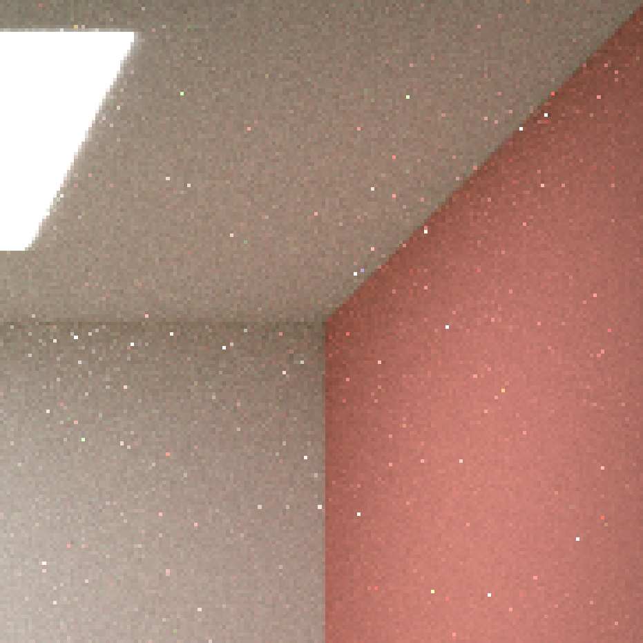
It is easy to see that the luminance blows up exponentially, why is that? The clue is in the coordiantes, the path keeps bouncing between the ceiling lamp and the ceiling itself, while keeping its X and Z coordinates relatively unchanged.

The ray marked with red eventually explodes. Expanding the sampling distribution offers an explanation:
$p(\omega_i) = \frac{1}{2\pi}$
Substituting this into the sample intensity equation:
$ \begin{aligned} I(\omega_i) = \rho L_i(x,\omega_i)*2cos(\theta_i) \end{aligned} $
When the input angle $\theta_i$ is small and the albedo ($\rho$) is larger than $0.5$ this can result in exponential growth:
$ \begin{aligned} I(\omega_i) = L_i(x,\omega_i)*X \end{aligned} $
Where $X>1$, potentially close to $2$.
This happens rarely, but when it does, the resulting sample has such high intensity that it leaves a bright sparkle behind on the rendered image. The algorithm still converges to the true value, but it needs exponentially many samples to correct one such rare mistake.
Cosine Weighted Hemisphere Sampling
What distribution should be used for the sampling then? Generally it should be as close to $g$ as possible. And in this case this easy to achieve. Solving
$ \begin{aligned} \frac{cos(\theta_i)}{\pi p(\omega_i)} = 1 \end{aligned} $
Gives us
$ \begin{aligned} p(\omega_i) = \frac{cos(\theta_i)}{\pi} \end{aligned} $
Which is luckily a probability density function already, namely it describes a cosine weighted hemisphere sampling. For futher reading on this I highly recommend Chapter 9 of Ray Tracing In One Weekend, which suggests an easy and robust approach for drawing samples from a cosine weighted hemisphere distribution around a given normal vector in code:
Vec3 cosineWeightedHemisphereSample(const Vec3 &normal, Rng &r)
{
    const auto v = uniformSphereSample(r);

    const auto direction = v + normal;

    return direction.normalized();
}
I find this method really elegant, here is a visualization of what is going on:

A uniform random direction ($r$) is chosen and added to the normal vector ($n$), the result ($s$) is then normalized.
With this approach we have:
$ \begin{aligned} I(\omega_i) = \rho L_i(x,\omega_i) \end{aligned} $
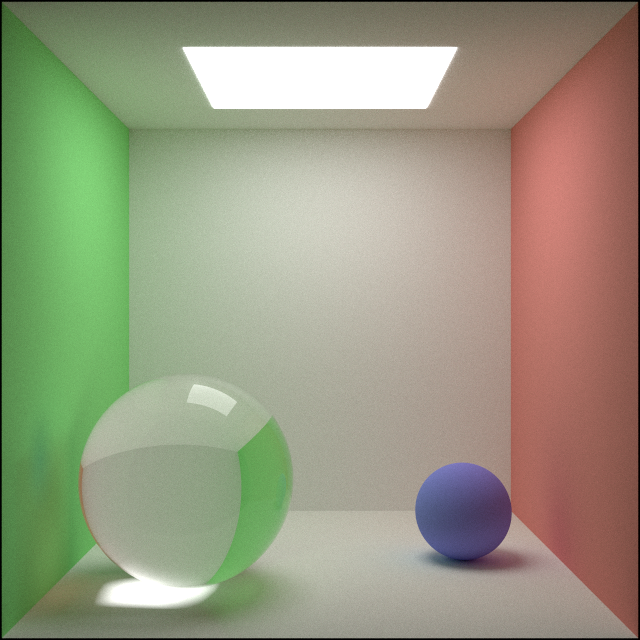
Using this function to for generating new directions gets rid of the annoying sparkles and even reduces noise:
Closing thoughts
I have pondered long about why these sparkles show up, looked through my code and logic many times to no avail. Sometimes things just work as intended, and it’s our expectation that is misplaced.
It is a really nice improvement both in that it improved the rendering out and also that I now udnerstand just how important it is to use the right sampler.
Next up I am planning to look at Next Event Estimation as an entry to Multiple Importance Sampling.